(This post is a bit herky-jerky… but, I’m trying to get better at just posting. Period)

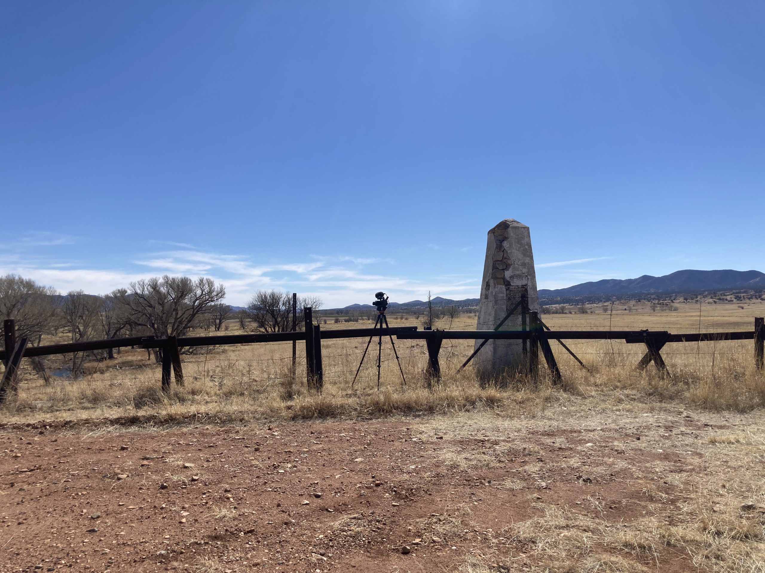
West of the Rio Grande, the border divide between the United States and Mexico is somewhat regularly studded with old, crumbling obelisks. One side is the United States of America. The other side is belongs to Los Estados Unidos Mexicanos – the United Mexican States. The middle of the marker is the carefully plotted dividing line between the two countries.
How was the dividing line decided? Coordinates, at that time in the late 1800’s, were determined by locating and plotting the stars. Each country created their own astronomical observatory camp, a momentous exercise that took a lot of planning, delicate instruments, mules, and people. The plan was the countries to compare their respective calculated coordinates and then try to split any difference.
The Mexican government was more organized and had a head start. As The Report of the Boundary Commission Survey and Remarking of the Boundary Between the United States and Mexico West of the Rio Grande 1891 to 1896 explained:
On the organization of the International Boundary Commission at Juarez, Mexico, November 17, 1891, the members of the Mexican section were present with a full outfit of instruments and observers ready for work.

These instruments had been purchased by the Mexican Government at the date of the first convention in 1892, and were used by them to determine the latitude and longitude of Juarez at that time while waiting for the United States Government to appoint a commission.

The United States commissioners having reached El Paso without instruments, men, or transportation, it was necessary for them to return north to organize their party, engage assistants, procure instruments, and purchase animals, wagons, and camp equipage before they would be able to begin field operations.

The time between December 1, 1891, and January 20, 1892, was spent in securing assistants and in organizing the transportation for the field parties.

The monuments are testaments of cooperation between the USA and Mexico. But, I had no idea about their existence until I started to encounter them during my film making.
The obelisks are often behind a USA-built border fence. Which is puzzling to me, since the fence is blocking off USA soil. Each country starts, from their respective sides of north or south, at the imaginary line dividing the middle of the monument.
MAPPING the BORDER MONUMENTS
I bump into the monuments, but could I seek them out? I wanted to have an easily accessible map.
The US side of the International Boundary and Water Commission has a GIS Portal. Using python, I downloaded a geojson and converted it to a kml file. Here a qre the border monuments if you’d like to play around with them!
I then uploaded the kml to my Gaia GPS app. I rarely have cell signal on the border and Gaia has the capability to pre-download maps, or any other feature you would like to know about in a signal-less land.
Below is the python code
import requests

# URL of the ArcGIS Feature Server query
url = "https://gisserver.ibwc.gov/agsserver/rest/services/USIBWCPublic/US_MexicoIBLandMonuments/FeatureServer/0/query?f=geojson&resultOffset=0&resultRecordCount=300&where=1%3D1&orderByFields=&outFields=*&returnGeometry=true&spatialRel=esriSpatialRelIntersects"

# Send a GET request to the URL
response = requests.get(url)

# Check if the request was successful
if response.status_code == 200:
    # Save the data to a file
    with open("monuments_ibwc.geojson", "w") as file:
        file.write(response.text)
    print("Data downloaded successfully.")
else:
    print(f"Failed to download data. Status code: {response.status_code}")
Data downloaded successfully.
import geopandas as gpd

# Load the GeoJSON file
gdf = gpd.read_file('monuments_ibwc.geojson')

# Display the first few rows of the GeoDataFrame
print(gdf.head())
  Monument DMS_Latitude_NAD83_CORS96 DMS_Longitude_NAD83_CORS96  \
0        1      N 31° 47' 02.00542''      W 106° 31' 47.07076''
1        2      N 31° 47' 02.00749''      W 106° 32' 14.12424''
2       2A      N 31° 47' 02.00665''      W 106° 32' 59.23714''
3       2B      N 31° 47' 02.00780''      W 106° 33' 24.56001''
4       2C      N 31° 47' 02.00874''      W 106° 34' 04.24815''

   Height_Meters  DD_Latitude_WGS84_Web_Mercator  \
0       1116.868                       31.783896
1       1287.742                       31.783896
2       1271.330                       31.783896
3       1159.515                       31.783896
4       1152.442                       31.783896

   DD_Longitude_WGS84_Web_Mercator   Last_Updated  \
0                      -106.529752  1706659200000
1                      -106.537267  1706659200000
2                      -106.549798  1706659200000
3                      -106.556832  1706659200000
4                      -106.567857  1706659200000

                                 GlobalID  OBJECTID  \
0  {9391E6C9-64D3-4825-87FB-13542DD07C0C}         1
1  {B5DAF77D-4AB9-4017-974F-777C3423A83C}         2
2  {27C4379F-5D84-4B01-A029-D2FC97B87670}         3
3  {47D5BEB2-0AFF-4C50-9255-DEAFACC6F85E}         4
4  {60230C00-6740-4A2D-8F4F-FF38C57D2A3D}         5

                     geometry
0  POINT (-106.52975 31.7839)
1  POINT (-106.53727 31.7839)
2   POINT (-106.5498 31.7839)
3  POINT (-106.55683 31.7839)
4  POINT (-106.56786 31.7839)
import geopandas as gpd
import folium
from folium import GeoJson, GeoJsonPopup, GeoJsonTooltip

# Load the GeoJSON file
gdf = gpd.read_file('monuments_ibwc.geojson')

# Create a base map centered around the GeoJSON data
m = folium.Map(location=[gdf.geometry.centroid.y.mean(), gdf.geometry.centroid.x.mean()], zoom_start=7)

# Define the popup and tooltip
popup = GeoJsonPopup(
    fields=["Monument"],
    aliases=["Monument:"],
    localize=True,
    labels=True,
    style="background-color: yellow;",
)

# Define the style function
def style_function(feature):
    return {
        "fillColor": "#000000",
        "color": "black",
        "weight": 2,
        "fillOpacity": 0.5,
    }

# Add the GeoJSON data to the map with the defined popup and tooltip
GeoJson(
    gdf,
    style_function=style_function,
    popup=popup,
).add_to(m)

# Save the map to an HTML file
m.save('map.html')

# Optionally, display the map in a Jupyter notebook
m
/var/folders/mg/ryc2w7fn6_5d8tpqzy55_g_40000gn/T/ipykernel_59475/3335339203.py:9: UserWarning: Geometry is in a geographic CRS. Results from 'centroid' are likely incorrect. Use 'GeoSeries.to_crs()' to re-project geometries to a projected CRS before this operation.

  m = folium.Map(location=[gdf.geometry.centroid.y.mean(), gdf.geometry.centroid.x.mean()], zoom_start=7)
## CONVERT TO KML
from pykml.factory import KML_ElementMaker as KML
from pykml.factory import GX_ElementMaker as GX
from lxml import etree

# Read the GeoJSON file
geojson_file = 'monuments_ibwc.geojson'
gdf = gpd.read_file(geojson_file)

# Create a KML document
kml_doc = KML.kml(
    KML.Document(
        *[KML.Placemark(
            KML.name(gdf.loc[i, 'Monument']),
            KML.Point(
                KML.coordinates(f"{gdf.geometry[i].x},{gdf.geometry[i].y}")
            )
        ) for i in range(len(gdf))]
    )
)

# Write the KML document to a file
kml_file = 'monuments_ibwc.kml'
with open(kml_file, 'wb') as f:
    f.write(etree.tostring(kml_doc, pretty_print=True, xml_declaration=True, encoding='UTF-8'))

print(f'GeoJSON file has been converted to KML file: {kml_file}')
GeoJSON file has been converted to KML file: monuments_ibwc.kml